
gpOptimizer: Single-Task#
## First, install the right version of gpCAM, and matplotlib
#!pip install gpcam==8.4.0
#!pip install matplotlib
Setup#
import numpy as np
import matplotlib.pyplot as plt
from gpcam import GPOptimizer
import time
from distributed import Client
client = Client()

%load_ext autoreload
%autoreload 2
from itertools import product
x_pred1D = np.linspace(0,1,1000).reshape(-1,1)
Data Prep#
x = np.linspace(0,600,1000)
def f1(x):
return np.sin(5. * x) + np.cos(10. * x) + (2.* (x-0.4)**2) * np.cos(100. * x)
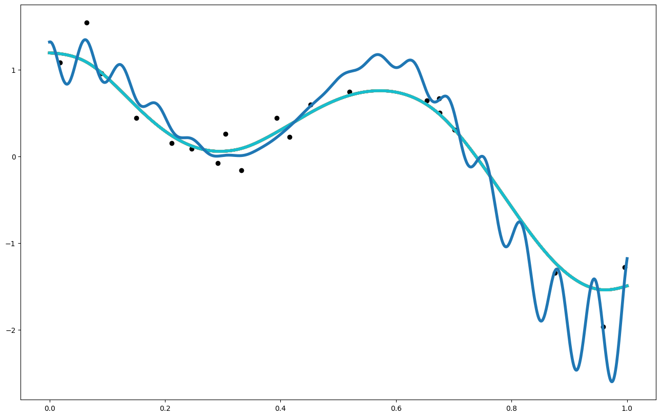
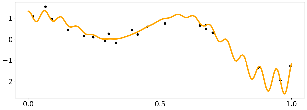
x_data = np.random.rand(20).reshape(-1,1)
y_data = f1(x_data[:,0]) + (np.random.rand(len(x_data))-0.5) * 0.5
plt.figure(figsize = (15,5))
plt.xticks([0.,0.5,1.0])
plt.yticks([-2,-1,0.,1])
plt.xticks(fontsize=20)
plt.yticks(fontsize=20)
plt.plot(x_pred1D,f1(x_pred1D), color = 'orange', linewidth = 4)
plt.scatter(x_data[:,0],y_data, color = 'black')
<matplotlib.collections.PathCollection at 0x7f85944cc150>
Customizing the Gaussian Process#
from gpcam.kernels import *
def my_noise(x,hps):
#This is a simple noise function, but can be arbitrarily complex using many hyperparameters.
#The noise function can return a matrix or a vector.
return np.zeros((len(x))) + hps[2]
#stationary
def skernel(x1,x2,hps):
#The kernel follows the mathematical definition of a kernel. This
#means there is no limit to the variety of kernels you can define.
d = get_distance_matrix(x1,x2)
return hps[0] * matern_kernel_diff1(d,hps[1])
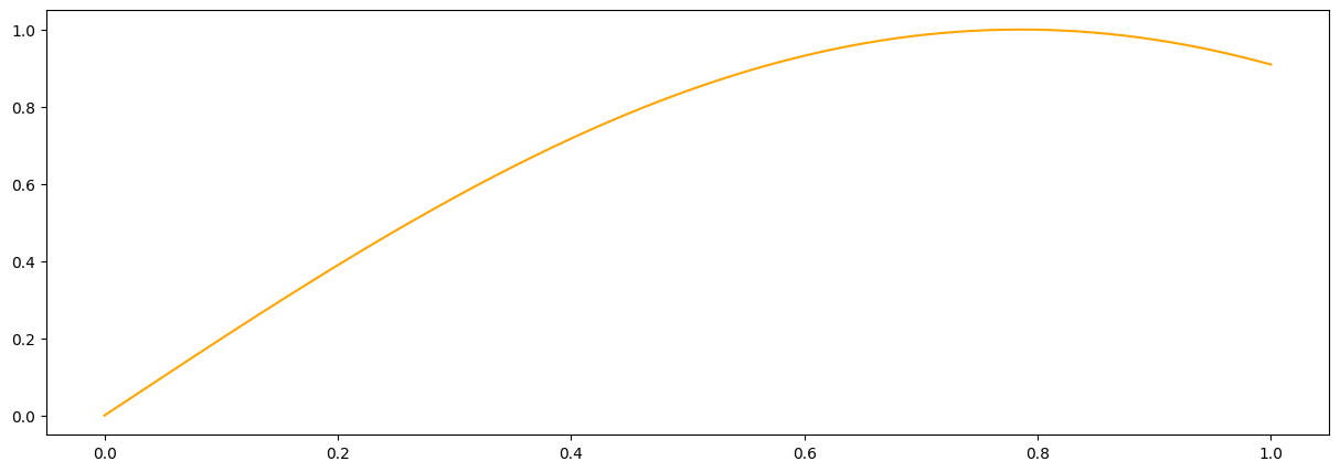
def meanf(x, hps):
#This ios a simple mean function but it can be arbitrarily complex using many hyperparameters.
return np.sin(hps[3] * x[:,0])
#it is a good idea to plot the prior mean function to make sure we did not mess up
plt.figure(figsize = (15,5))
plt.plot(x_pred1D,meanf(x_pred1D, np.array([1.,1.,5.0,2.])), color = 'orange', label = 'task1')
[<matplotlib.lines.Line2D at 0x7f859445db90>]
Initialization and Different Training Options#
my_gpo = GPOptimizer(x_data,y_data,
            init_hyperparameters = np.ones((4))/10.,  # We need enough of those for kernel, noise, and prior mean functions
            noise_variances=np.ones(y_data.shape) * 0.01, # providing noise variances and a noise function will raise a warning
            compute_device='cpu',
            kernel_function=skernel,
            kernel_function_grad=None,
            prior_mean_function=meanf,
            prior_mean_function_grad=None,
            gp2Scale = False,
            ram_economy=False,
            args=None,
            )

hps_bounds = np.array([[0.01,10.], #signal variance for the kernel
                       [0.01,10.], #length scale for the kernel
                       [0.001,1.],  #noise
                       [0.01,1.]  #mean
                      ])

x_update = np.array([0.1,0.2,0.5]).reshape(3,1)
y_update = f1(x_update[:,0]) + (np.random.rand(len(x_update))-0.5) * 0.5
my_gpo.tell(x_update,
            y_update,
            noise_variances=np.ones(y_update.shape) * 0.05,
            append=True, rank_n_update=True)


st = time.time()
print("Standard Training (MCMC)")
hps = my_gpo.train(hyperparameter_bounds=hps_bounds, info = False)
print("Result=", hps, "after ", time.time() - st, " seconds")
print("ML: ",my_gpo.log_likelihood())
print("")

print("ADAM")
hps = my_gpo.train(hyperparameter_bounds=hps_bounds, info = True, max_iter = 100, method="adam")
print("Result=", hps, "after ", time.time() - st, " seconds")
print("ML: ",my_gpo.log_likelihood())
print("")

print("Global Training")
hps = my_gpo.train(hyperparameter_bounds=hps_bounds, method='global', max_iter = 20)
print("Result=", hps, "after ", time.time() - st, " seconds")
print("ML: ",my_gpo.log_likelihood())
print("")

print("Local Training")
hps = my_gpo.train(hyperparameter_bounds=hps_bounds, method='local')
print("Result=", hps, "after ", time.time() - st, " seconds")
print("ML: ",my_gpo.log_likelihood())
print("")

print("HGDL Training")
hps = my_gpo.train(hyperparameter_bounds=hps_bounds, method='hgdl', max_iter=2, dask_client=client)
print("Result=", hps, "after ", time.time() - st, " seconds")
print("ML: ",my_gpo.log_likelihood())
print("")
Standard Training (MCMC)
Result= [1.42043585 0.18136244 0.63264998 0.3994427 ] after  2.0698695182800293  seconds
ML:  -13.73108037276967

ADAM
Result= [ 0.62067829  0.10733495  0.63264998 -0.48495006] after  2.1269960403442383  seconds
ML:  -12.38927498851401

Global Training
Result= [0.71603223 0.11839417 0.31018575 0.01230455] after  2.3952267169952393  seconds
ML:  -12.775291643017294

Local Training
Result= [0.71704799 0.11777473 0.31018575 0.01229138] after  2.3981099128723145  seconds
ML:  -12.774267386444588

HGDL Training
Result= [0.72461375 0.11705147 0.16345602 0.01      ] after  3.2672066688537598  seconds
ML:  -12.770394933400771
my_gpo.get_data().keys()
dict_keys(['input dim', 'x data', 'y data', 'measurement variances', 'hyperparameters', 'cost function'])
Asynchronous Training#
Train asynchronously – via Adam, HGDL, or MCMC – on a remote server or locally. You can also start a bunch of different training runs on different computers. This training will continue without any signs of life until you query the solution via ‘update_hyperparameters(object)’ or call ‘my_gpo.stop_training(opt_obj)’
HGDL#
my_gpo.set_hyperparameters(np.array([1.,1.,1.,1.]))
print(my_gpo.hyperparameters)
opt_obj = my_gpo.train(hyperparameter_bounds=hps_bounds, dask_client=client, asynchronous=True, method='hgdl')
# The result won't change much (or at all) since this is such a simple optimization
for i in range(20):
    my_gpo.update_hyperparameters(opt_obj)
    print("iteration ", i, " : ",my_gpo.hyperparameters)
    time.sleep(0.1)
my_gpo.stop_training(opt_obj) ##this leaves the dask client alive, kill_client() will shut it down.
[1. 1. 1. 1.]
iteration  0  :  [1. 1. 1. 1.]
iteration  1  :  [0.72461379 0.11705147 0.33091475 0.01      ]
/home/marcus/Coding/fvGP/fvgp/gp.py:881: UserWarning: Hyperparameter update not successful len(optima list) = 0
  hps = self.trainer.update_hyperparameters(opt_obj)
iteration  2  :  [0.72461379 0.11705147 0.33091475 0.01      ]
iteration  3  :  [0.72461379 0.11705147 0.33091475 0.01      ]
iteration  4  :  [0.72461379 0.11705147 0.33091475 0.01      ]
iteration  5  :  [0.72461379 0.11705147 0.33091475 0.01      ]
iteration  6  :  [0.72461379 0.11705147 0.33091475 0.01      ]
iteration  7  :  [0.72461379 0.11705147 0.33091475 0.01      ]
iteration  8  :  [0.72461379 0.11705147 0.33091475 0.01      ]
iteration  9  :  [0.72461379 0.11705147 0.33091475 0.01      ]
iteration  10  :  [0.72461379 0.11705147 0.33091475 0.01      ]
iteration  11  :  [0.72461379 0.11705147 0.33091475 0.01      ]
iteration  12  :  [0.72461379 0.11705147 0.33091475 0.01      ]
iteration  13  :  [0.72461379 0.11705147 0.33091475 0.01      ]
iteration  14  :  [0.72461379 0.11705147 0.33091475 0.01      ]
iteration  15  :  [0.72461379 0.11705147 0.33091475 0.01      ]
iteration  16  :  [0.72461379 0.11705147 0.33091475 0.01      ]
iteration  17  :  [0.72461379 0.11705147 0.33091475 0.01      ]
iteration  18  :  [0.72461379 0.11705147 0.33091475 0.01      ]
iteration  19  :  [0.72461379 0.11705147 0.33091475 0.01      ]
ADAM#
my_gpo.set_hyperparameters(np.array([1.,1.,1.,1.]))
print(my_gpo.hyperparameters)
opt_obj = my_gpo.train(hyperparameter_bounds=hps_bounds, dask_client=client, asynchronous=True, method='adam')
# The result won't change much (or at all) since this is such a simple optimization
for i in range(20):
    my_gpo.update_hyperparameters(opt_obj)
    print("iteration ", i, " : ",my_gpo.hyperparameters)
    time.sleep(0.1)
my_gpo.stop_training(opt_obj) ##this leaves the dask client alive, kill_client() will shut it down.
[1. 1. 1. 1.]
iteration  0  :  [1. 1. 1. 1.]
iteration  1  :  [1.5182732  0.16176409 1.         0.06287896]
iteration  2  :  [ 1.30248894  0.15005184  1.         -0.42165649]
iteration  3  :  [ 0.97456699  0.13062211  1.         -0.50436911]
iteration  4  :  [ 0.67331715  0.11093058  1.         -0.52952518]
iteration  5  :  [ 0.63166861  0.10807816  1.         -0.53260203]
iteration  6  :  [ 0.63138508  0.10805866  1.         -0.53262287]
iteration  7  :  [ 0.63138508  0.10805866  1.         -0.53262287]
iteration  8  :  [ 0.63138508  0.10805866  1.         -0.53262287]
iteration  9  :  [ 0.63138508  0.10805866  1.         -0.53262287]
iteration  10  :  [ 0.63138508  0.10805866  1.         -0.53262287]
iteration  11  :  [ 0.63138508  0.10805866  1.         -0.53262287]
iteration  12  :  [ 0.63138508  0.10805866  1.         -0.53262287]
iteration  13  :  [ 0.63138508  0.10805866  1.         -0.53262287]
iteration  14  :  [ 0.63138508  0.10805866  1.         -0.53262287]
iteration  15  :  [ 0.63138508  0.10805866  1.         -0.53262287]
iteration  16  :  [ 0.63138508  0.10805866  1.         -0.53262287]
iteration  17  :  [ 0.63138508  0.10805866  1.         -0.53262287]
iteration  18  :  [ 0.63138508  0.10805866  1.         -0.53262287]
iteration  19  :  [ 0.63138508  0.10805866  1.         -0.53262287]
MCMC#
my_gpo.set_hyperparameters(np.array([1.,1.,1.,1.]))
print(my_gpo.hyperparameters)
opt_obj = my_gpo.train(hyperparameter_bounds=hps_bounds, dask_client=client, asynchronous=True, method='mcmc')
# The result won't change much (or at all) since this is such a simple optimization
for i in range(20):
    my_gpo.update_hyperparameters(opt_obj)
    print("iteration ", i, " : ",my_gpo.hyperparameters)
    time.sleep(0.1)
my_gpo.stop_training(opt_obj) ##this leaves the dask client alive, kill_client() will shut it down.
[1. 1. 1. 1.]
iteration  0  :  [1. 1. 1. 1.]
iteration  1  :  [0.50370854 0.15573954 0.7384795  0.68431549]
iteration  2  :  [1.86428506 0.18317467 0.64664979 0.94843172]
iteration  3  :  [1.14175814 0.09617595 0.5580199  0.96909571]
iteration  4  :  [1.12777223 0.13854249 0.38769585 0.97151315]
iteration  5  :  [1.43008675 0.21813723 0.26743826 0.90153651]
iteration  6  :  [2.14864015 0.24951402 0.29146359 0.90941524]
iteration  7  :  [2.71848843 0.23041502 0.34257909 0.93758508]
iteration  8  :  [3.08285914 0.35745852 0.16746233 0.95074552]
iteration  9  :  [2.18294056 0.21796311 0.02209146 0.82927373]
iteration  10  :  [1.68086173 0.19758897 0.13361436 0.60215922]
iteration  11  :  [1.70172816 0.17342578 0.01829901 0.34949083]
iteration  12  :  [0.97540374 0.1247531  0.23000177 0.38452528]
iteration  13  :  [0.89779387 0.16397485 0.31150347 0.52650927]
iteration  14  :  [2.01123233 0.26928425 0.20814976 0.40257825]
iteration  15  :  [1.79071559 0.18325646 0.13083905 0.6360191 ]
iteration  16  :  [0.80741772 0.17267156 0.06504115 0.61579112]
iteration  17  :  [0.79417929 0.13135874 0.03150897 0.5702635 ]
iteration  18  :  [0.79417929 0.13135874 0.03150897 0.5702635 ]
iteration  19  :  [0.79417929 0.13135874 0.03150897 0.5702635 ]
Plotting the Result#
#let's make a prediction
x_pred = np.linspace(0,1,1000)
hps = my_gpo.train(hyperparameter_bounds=hps_bounds, info = False)
# different ways to call
var1 = my_gpo.posterior_covariance(x_pred.reshape(-1,1), variance_only=False, add_noise=False)["v(x)"]
var1 = my_gpo.posterior_covariance(x_pred.reshape(-1,1), variance_only=False, add_noise=True)["v(x)"]
mean1 = my_gpo.posterior_mean(x_pred.reshape(-1,1))["m(x)"]
var1 = my_gpo.posterior_covariance(x_pred.reshape(-1,1), variance_only=False, add_noise=True)["v(x)"]
mean_grad = my_gpo.posterior_mean_grad(x_pred.reshape(-1,1), direction=0)["dm/dx"]
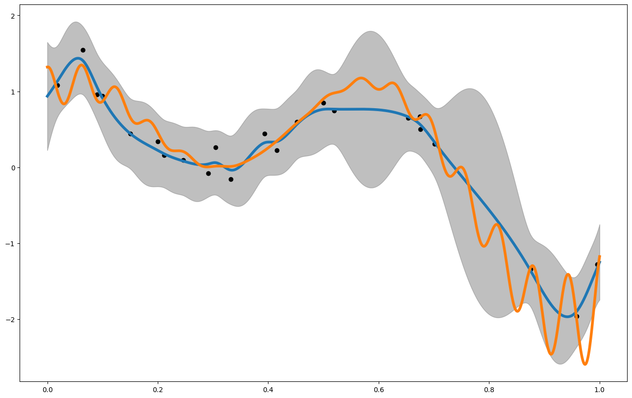
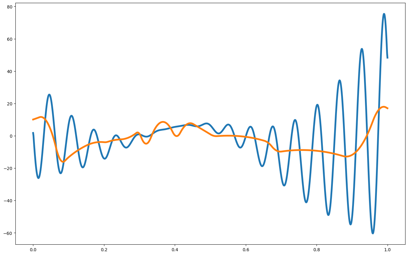
print("Posterior Mean and Uncertainty")
plt.figure(figsize = (16,10))
plt.plot(x_pred,mean1, label = "posterior mean", linewidth = 4)
plt.plot(x_pred1D,f1(x_pred1D), label = "latent function", linewidth = 4)
plt.fill_between(x_pred, mean1 - 3. * np.sqrt(var1), mean1 + 3. * np.sqrt(var1), alpha = 0.5, color = "grey", label = "var")
plt.scatter(my_gpo.x_data,my_gpo.y_data, color = 'black')
plt.show()
print("Posterior Mean Gradient")
plt.figure(figsize = (16,10))
dx = 1./len(x_pred)
plt.plot(x_pred1D,np.gradient(f1(x_pred1D).flatten(), dx), label = "ground truth gradient", linewidth = 4)
plt.plot(x_pred1D,mean_grad, label = "posterior mean grad", linewidth = 4)
plt.show()
##looking at some validation metrics
print("RMSE: ",my_gpo.rmse(x_pred1D,f1(x_pred1D).flatten()))
print("NRMSE: ",my_gpo.nrmse(x_pred1D,f1(x_pred1D).flatten()))
print("CRPS (mean, std): ",my_gpo.crps(x_pred1D,f1(x_pred1D).flatten()))
print("R2: ",my_gpo.r2(x_pred1D,f1(x_pred1D).flatten()))
print("NLPD: ",my_gpo.nlpd(x_pred1D,f1(x_pred1D).flatten()))
print("MSLL: ",my_gpo.msll(x_pred1D,f1(x_pred1D).flatten()))
print("MAPE: ",my_gpo.mape(x_pred1D,f1(x_pred1D).flatten()))
print("INTERVAL SCORE: ",my_gpo.interval_score(x_pred1D,f1(x_pred1D).flatten()))
print("MPIW: ",my_gpo.mpiw(x_pred1D))
print("PICP: ",my_gpo.picp(x_pred1D,f1(x_pred1D).flatten()))
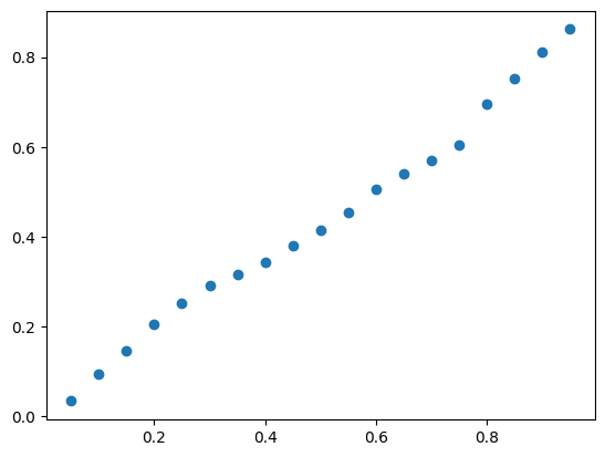
print("Coverage Curve:")
cov_curve = my_gpo.coverage_curve(x_pred1D,f1(x_pred1D).flatten())
plt.scatter(cov_curve["target_coverage"], cov_curve["measured_coverage"])
plt.show()
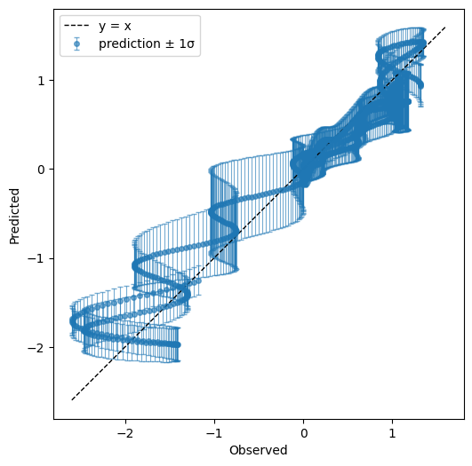
print("predicted vs. observed")
my_gpo.plot_observed_vs_predicted(x_pred1D,f1(x_pred1D).flatten())
Posterior Mean and Uncertainty
Posterior Mean Gradient
RMSE:              0.2912545093455239
NRMSE:             0.07384928463520797
CRPS (mean, std):  (np.float64(0.16466760019121685), np.float64(0.16053216387850855))
R2:                0.9203225767967481
NLPD:              1.181955347249296
MSLL:              -0.37194114389288413
MAPE:              0.980544266141841
INTERVAL SCORE:    1.8226636504364473
MPIW:              0.8112905431811624
PICP:              0.862
Coverage Curve:
predicted vs. observed
#We can ask mutual information and total correlation there is given some test data
x_test = np.array([[0.45],[0.45]])
print("Mutual Information: ",my_gpo.gp_mutual_information(x_test))
print("Total Correlation : ",my_gpo.gp_total_correlation(x_test))
Mutual Information:  {'x': array([[0.45],
       [0.45]]), 'mutual information': np.float64(5.437073730749979)}
Total Correlation :  {'x': array([[0.45],
       [0.45]]), 'total correlation': np.float64(16.418699956034402)}
next_point = my_gpo.ask(np.array([[0.,1.]]))
print(next_point)
{'x': array([[0.78929474]]), 'f_a(x)': array([0.44872093]), 'opt_obj': None}
Running many GPs at once in parallel#
#duplicate data: in practice, this would be different data in every column
y_data = np.broadcast_to(y_data[:, None], (y_data.size, 10))

my_gpo = GPOptimizer(x_data,y_data,
            init_hyperparameters = np.ones((2))/10.,  # we need enough of those for kernel, noise, and prior mean functions
            noise_variances=np.ones(y_data.shape[0]) * 0.1, # providing noise variances and a noise function will raise a warning
            compute_device='cpu',
            )


hps_bounds = np.array([[0.01,10.], #signal variance for the kernel
                       [0.01,10.], #length scale for the kernel
                      ])

print("Standard Training (MCMC)")
hps = my_gpo.train(hyperparameter_bounds=hps_bounds, info = True, max_iter = 100)
print("Result=", hps, "after ", time.time() - st, " seconds")
print("")
Standard Training (MCMC)
Starting likelihood. f(x)=  -22.80247881875027
Finished  10  out of  100  iterations. f(x)=  -12.56523120782898
Finished  20  out of  100  iterations. f(x)=  -12.62131433421405
Finished  30  out of  100  iterations. f(x)=  -12.432843037484474
Finished  40  out of  100  iterations. f(x)=  -12.672321392442349
Finished  50  out of  100  iterations. f(x)=  -14.104788430403184
Finished  60  out of  100  iterations. f(x)=  -12.766945819780151
Finished  70  out of  100  iterations. f(x)=  -12.98159622712429
Finished  80  out of  100  iterations. f(x)=  -12.04808211364757
Finished  90  out of  100  iterations. f(x)=  -12.553768629893241
Result= [0.93037651 0.31860921] after  20.719249486923218  seconds
x_pred = np.linspace(0,1,1000).reshape(1000,1)
mean = my_gpo.posterior_mean(x_pred)["m(x)"]
sd   = np.sqrt(my_gpo.posterior_covariance(x_pred)["v(x)"])
print("Posterior Means and Uncertainties")
plt.figure(figsize = (16,10))
for i in range(10):
    plt.plot(x_pred.flatten(),mean[:,i], label = "posterior mean", linewidth = 4)
plt.scatter(my_gpo.x_data,my_gpo.y_data[:,0], color = 'black')
plt.plot(x_pred1D,f1(x_pred1D), label = "latent function", linewidth = 4)
plt.show()
Posterior Means and Uncertainties